
Overview
AMPT is an online platform to perform sample size and power calculations for precision medicine trials in mental health and other indications.
Available Designs:
- Standard biomarker-based designs (Randomize-all, Enrichment, Strategy)
- Generalized Randomized Basket design with an Interim Analysis (GRaBiT)
- Sequential Multiple Assignment Randomized Trial with Internal Pilot and Sample size Re-estimation (SMARTIES)
Overview of Trial Design Types:
• Randomize-All — Randomize all participants regardless of biomarker status.
• Enrichment — Screen and randomize only biomarker-positive (M+) participants.
• Strategy — Randomize participants to receive control treatment regardless of biomarker status, versus a precision treatment approach where M+ and M− participants receive experimental and control treatments, respectively.
Overview of GRaBIt:
Randomized basket trials test a common treatment vs. control across several related diseases. The GRaBIt design improves on prior basket methods by allowing each disease subgroup (basket) to have different sample sizes and treatment effects. The trial proceeds in two stages. In Stage 1, a fraction of participants are enrolled and randomized in each disease subgroup (basket). We perform an interim analysis to identify and remove baskets in which the experimental treatment is not efficacious. In Stage 2, the participants in the remaining baskets are enrolled and we perform a final pooled analysis of Stage 1 and Stage 2 data from the remaining baskets only. The trial tests whether the experimental treatment is superior to control in selected disease subgroups (baskets).
Randomized basket trials test a common treatment vs. control across several related diseases. The GRaBIt design improves on prior basket methods by allowing each disease subgroup (basket) to have different sample sizes and treatment effects. The trial proceeds in two stages. In Stage 1, a fraction of participants are enrolled and randomized in each disease subgroup (basket). We perform an interim analysis to identify and remove baskets in which the experimental treatment is not efficacious. In Stage 2, the participants in the remaining baskets are enrolled and we perform a final pooled analysis of Stage 1 and Stage 2 data from the remaining baskets only. The trial tests whether the experimental treatment is superior to control in selected disease subgroups (baskets).
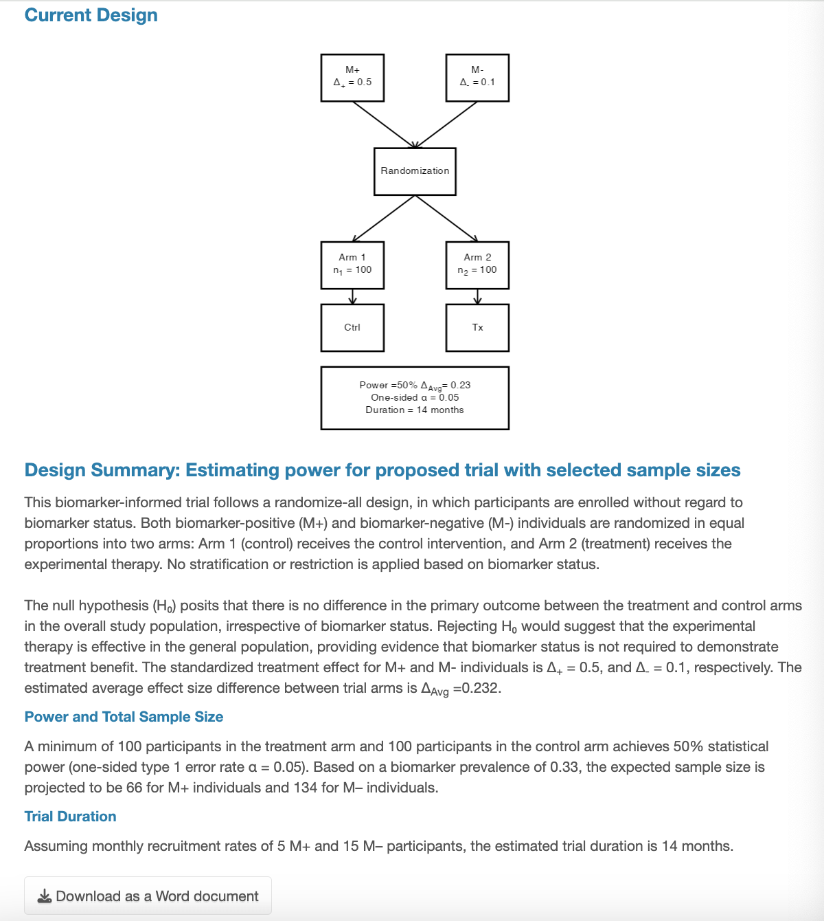
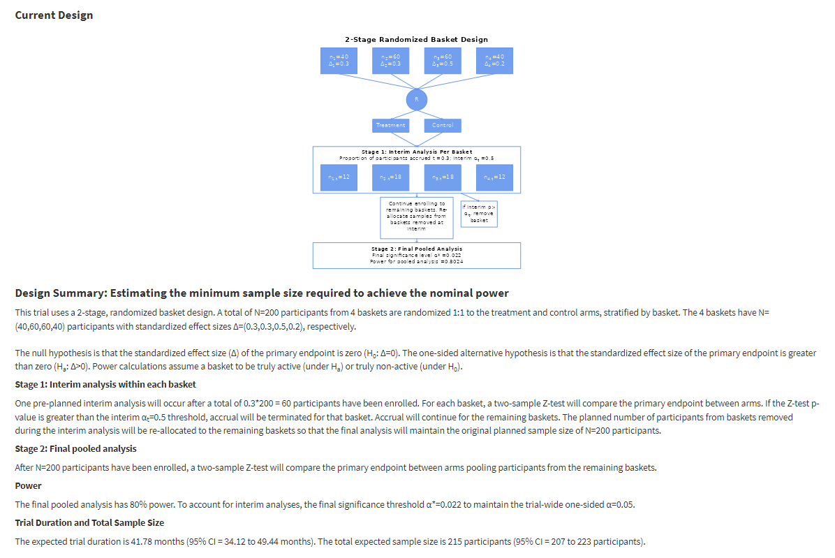
Current Design
Design Summary: Estimating the minimum sample size required to achieve the nominal power
Design Summary: Estimating power for proposed trial with selected sample sizes
Stage 1: Interim analysis within each basket
Stage 2: Final pooled analysis
Power
Trial Duration and Total Sample Size
SMARTIES
Designing SMARTs with Internal Pilot
and Unblinded Sample Size Re-estimation
and Unblinded Sample Size Re-estimation
An online tool for designing Sequential Multiple Assignment Randomized Trials with an internal pilot study and unblinded sample size re-estimation.
New features
Stage 1
Randomization
Randomization
Responder
Non-responder
Stage 2
Randomization
Randomization
Internal Pilot
Feasibility
Assessment
Feasibility
Assessment
Sample Size
Re-estimation
Re-estimation
Interim Decision
/ Adjustment
/ Adjustment
Continue Trial
with Adaptation
with Adaptation
Overview
SMARTIES is an online tool for designing Sequential Multiple Assignment Randomized Trials with an internal pilot study and unblinded sample size re-estimation (SMARTIES). It supports feasibility assessment, interim decision-making, and sample size planning for stage-specific SMART analyses.
Key Functions
- Support internal pilot feasibility assessment, interim decision-making, and unblinded sample size re-estimation for SMART designs
- Downloadable report with study schema and protocol summary
- Detailed documentation and step-by-step tutorial to aid users


Step 1: Internal Pilot Study (Phase I) Design for Testing Feasibility
Step 2: Initial Main Trial (Phase II) Design for Testing Efficacy
Step 3: Final Design after Interim Analysis with Sample Size Re-estimation (SSR)
Output after interim sample size re-estimation
Decision Rule (CHW)
Distribution of main output
Interpretation
Trial Schema and Final Summary
Trial Schema
Standard Designs Documentation
There are three available standard designs:
1. Randomize-All Design:
All eligible participants are randomized to treatment vs. control regardless their biomarker status.
The trial tests whether the treatment is efficacious across all participants.
2. Enrichment Design:
All eligible participants are first screened for the selected biomarker.
Only participants who screen positive for the biomarker (M+) are randomized to treatment vs. control.
The trial tests whether the treatment is efficacious in M+ participants only.
3. Strategy Design:
All eligible participants are first screened for the selected biomarker.
Participants are randomized to either a “biomarker-based strategy”
(where M+ and M- participants receive the experimental or control treatments,
respectively) or to a “biomarker-agnostic strategy” (where all participants receive the control treatment).
The trial tests whether using the biomarker-based strategy to guide treatment improves outcomes.
Standard Designs
Inputs Panel
Sample size of arm1 := The number of participants in arm 1 (control).
Targeted power := designated \(1-\beta\) level for the entire trial. One minus the type II error rate.
Standardized effect size for M+ patients (Δ+) := The expected standardized effect size for biomarker positive population.
Standardized effect size for M- patients (Δ-) := The expected standardized effect size for biomarker negative population.
Biomarker prevalence := proportion of general population that are biomarker positive.
Hypothesis Test := Two-sided tests evaluate a null hypothesis of equality, while one-sided tests evaluate a null hypothesis with a greater-than or less-than condition.
Significance level (\(\alpha\)) := designated \(\alpha\) level for the entire trial, false positive rate overall.
Randomization ratio (Arm 2 / Arm 1) := Allocation ratio of arm 2 (strategy/treatment) to arm 1 (control).
Accrual rate of M+ participants (pts/month) := Accrual rate of biomarker-positive (M⁺) individuals per month.
Accrual rate of M- participants (pts/month) := Accrual rate of biomarker-negative (M⁻) individuals per month.
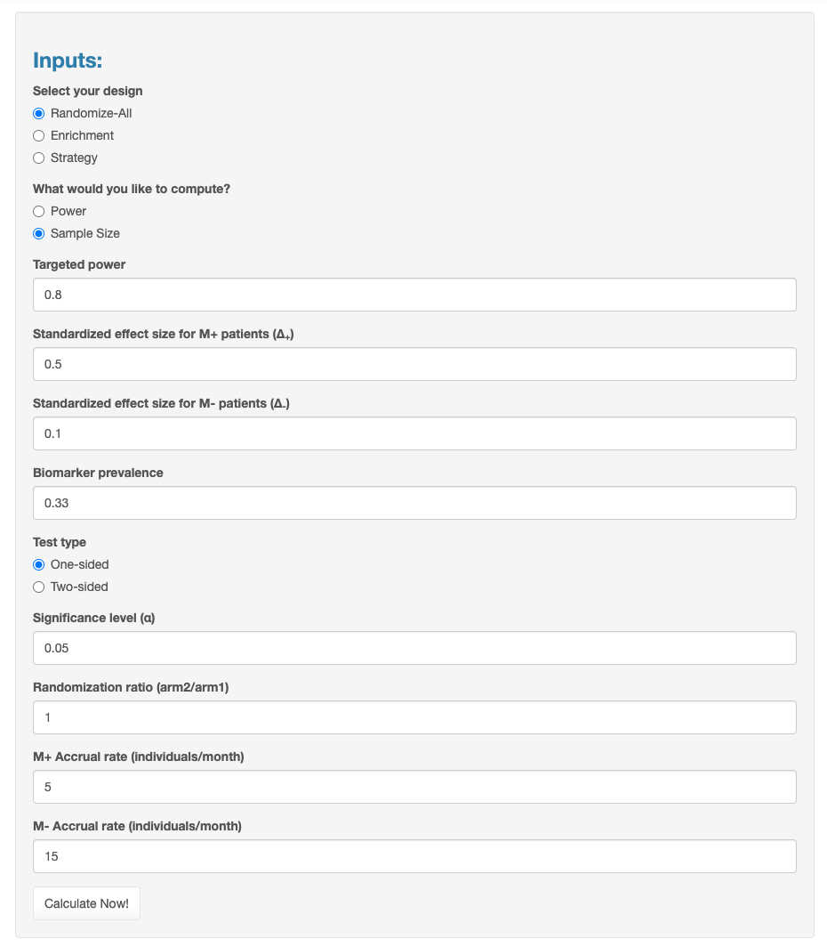
Click Calculate Now! to view outputs.
Outputs Panel
Current Design
An illustration produced to show the current design of the trail based on your inputs. To copy, simply right click>"copy image"or"save image as". If texts are not fitting well, please adjust the width of you browser until it fits properly.
Design Summary
A test summary of current design of the trial based on your inputs. You can directy copy it since it is in text format.
Download as a Word Document
Click here to download all the content above, including text, images, and formatting, as a Word document.
GRaBIt Documentation
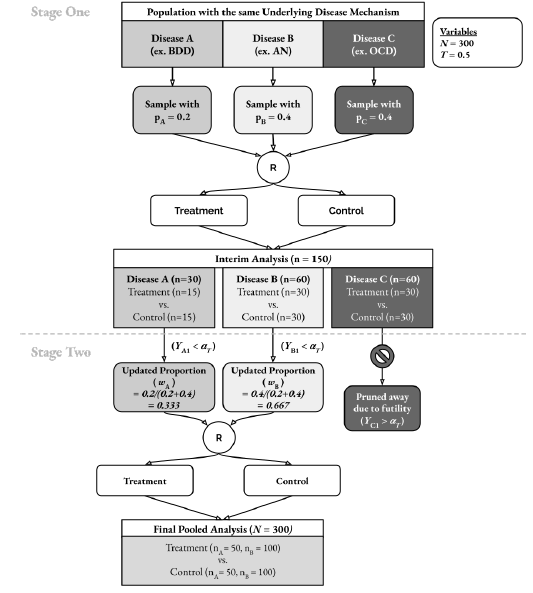
Above is a motivating example from Patel (2024). We obtain key metrics such as the total sample size for each basket, the true activity status of each basket, and the proportion of participants accrued during the interim analysis. To tailor the analysis to their specific trial designs, users provide additional inputs. This ensures maximum flexibility when computing test statistics. Refer to the screenshot below for guidance on transcribing the design above into inputs.
Inputs Panel
Vector Inputs (Multiple Values):
Total sample size of each basket := The number of participants per basket, using only commas to separate them. Ensure they are all positive even integers, so that after randomization, the cohort sizes in both the treatment and control arms are whole numbers. The length of the input vector corresponds to the number of baskets.
Relative ratio of each basket := The relative ratio of sample size in each basket, in the same order & format as above. Investigator can estimate effect sizes from published results.
Standardized effect size(\(\Delta\)) of each basket := The expected effect size per basket, in the same order & format as above. Investigator can estimate this ratio via subtype prevalence from published results.
Accrual rate (individual/month) of each basket := number of individuals recruited per month in each basket, in the same order & format as the sample size input above.
Scalar Inputs(Single Value):
Nominal power := designated \(1-\beta\) level for the entire trial. One minus the type II error rate.
Proportion of participants accrued at interim analysis(\(t\)) := Interim analysis cutoff point, or % of total amount of participants recruited. This ratio should be consistent across all baskets.
Interim significance level(\(\alpha_t\)) := designated \(\alpha\) level for the interim analysis at proportion t. The basket with a p-value larger than this threshold will be dropped.
Trial-wide significance level(\(\alpha\)) := designated \(\alpha\) level for the entire trial, false positive rate overall.
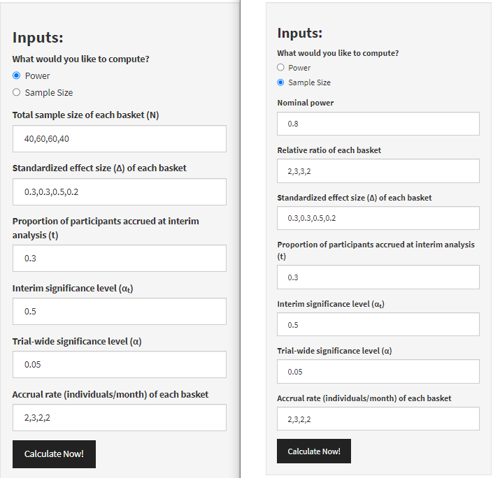
Once all inputs have been filled as desired and vector inputs are ensured to be of the same length, click Calculate Now! to view outputs.
Outputs Panel
Current Design
An illustration produced to show the current design of the trail based on your inputs. To copy, simply right click>"copy image"or"save image as". If texts are not fitting well, please adjust the width of you browser until it fits properly.
Design Summary
A test summary of current design of the trial based on your inputs. You can directy copy it since it is in text format.
Download as a Word Document
Click here to download all the content above, including text, images, and formatting, as a Word document.
A Glimpse of the Statistical Method
For detailed deriviation, please refer to Patel 2024 paper in the references.
Trial-wide Type 1 Error Rate:
\( \alpha = \sum_{m}Pr_{H_0}(V_m|\alpha^*,\alpha_t,m,\Delta)= \sum_{m}Pr_{H0}(\cap_{\,i\in id(m)}Y_{i1}>Z_{1-\alpha_t},V_m>Z_{1-\alpha^*})\cdot(1-\alpha_t)^{K-|id(m)|} \)
The overall type 1 error rate is a summed rejection probability under the null of different built, the rejection probability is assessed whether all baskets passing through interim and final stage.
Power
\( 1- \beta = \sum_{m}Pr_{H_{1g}}(V_m|\alpha^*,\alpha_t,m,\Delta) \)
Similarly, The power is a summed rejection probability under the alternative of different built.
SMARTIES Documentation
SMARTIES is a two phase adaptive design with an internal pilot study for feasibility assessment and unblindedc sample size re-estimation (Phase I), followed by a main trial for testing efficacy with adjusted sample size when needed (Phase II).
Quick Start
- Step 1 (Feasibility): Enter p0, p1, α, target power, and number of candidate designs. Choose Auto/Manual and click
Use this designto lock the internal pilot design. - Step 2 (Initial main trial sample size calculation): Enter α, power, SD, and planned mean difference d. Click
Lock original main trial sample sizeto lock Norig. - Step 3 (SSR): Enter dobs, γl, γu, nsims, seed, then click
Run Sample Size Re-estimation. - Report: Review the final summary and click
Download Word report.
Step 1: Internal Pilot (Feasibility)
Goal: decide whether the trial is feasible to proceed based on a one-stage exact test for a binary feasibility endpoint.
- p0: unacceptable feasibility success rate.
- p1: acceptable feasibility success rate (must satisfy p1 > p0).
- α (one-sided): Type I error for feasibility test.
- Power: probability of declaring feasibility under p1.
- Output: interim total sample size nint and feasibility cutoff rfeas.
Step 2: Initial Main Trial (Efficacy)
Goal: compute the initial planned sample size for a two-arm superiority test under user-specified α, power, SD, and planned mean difference d.
- Output: per-arm norig and total Norig.
- Tip: ensure per-arm interim n (from Step 1) is smaller than per-arm planned n (from Step 2) so the interim information fraction is valid.
Step 3: SSR using the CHW conditional power rule
Goal: re-estimate the required sample size based on conditional power computed from interim data.
Key quantities
- dobs: observed interim mean difference (user input).
- t: interim information fraction (approximately nint/2 divided by norig).
- CPplan: conditional power under planned effect size.
- CPobs: conditional power under observed interim effect size.
- γl, γu: lower/upper thresholds defining zones.
Decision zones (CHW)
- Futility: CPobs < γl × CPplan (keep original N; consider stopping).
- Promising: γl × CPplan ≤ CPobs ≤ γu × CPplan (apply CHW inflation / top-up).
- Success: CPobs > γu × CPplan (keep original N).
The app summarizes SSR via simulation (nsims runs), producing the distribution of suggested N and the zone proportions.
How to read the outputs
- Design header: locked Step 1/2 inputs, final α, and interim t.
- Key metrics table: effect sizes, CP metrics, and suggested sample size summary.
- Decision rule & interpretation: CHW rule + dominant zone statement.
- Plots: zone counts + histogram of suggested total N.
- Word report: timestamp + summary + rule + schema figure.
Our Team

Contact:
For assistance, please contact Dr. Clement Ma clement.ma@camh.ca.
Funding:
This project has been funded by the Ontario Brain Institute Centre for Analytics and the CAMH Discovery Fund.
If you are using this APP, please cite the relevant reference(s) according to your study design:
- Standard design → cite #1 and #4
- GRaBIt → cite #2 and #4
- SMARTIES → cite #3 and #5
References
- Wu, X., Patel, S. S., Szatmari, P., Rajji, T., Husain, M. I., Castle, D., & Ma, C. (2026). Biomarker-based study designs for precision psychiatry trials [Manuscript under review].
- Patel, S. S., Chen, D. Z., Castle, D., & Ma, C. (2024). Randomized basket trial with an interim analysis (RaBIt) and applications in mental health (arXiv preprint). https://arxiv.org/abs/2411.13692
- [Placeholder for SMARTIES method reference]
- Chen, D. Z., Xie, A., & Ma, C. (2026). Accelerating mental health precision trial: An effective visualization-driven tool for power and sample size estimation in biomarker-based study designs [Preprint]. medRxiv. https://doi.org/10.64898/2026.05.06.26352613
- Xie, A., Chen, D. Z., & Ma, C. (2026). RShiny app for designing sequential multiple assignment randomized trial designs with internal pilot study and unblinded sample size re-estimation [Manuscript in preparation].